Introduction

Statistical hypothesis testing is a fundamental component of biological research. Researchers frequently need to determine whether the mean value observed in a sample differs significantly from a known or expected population value. In such situations, the One Sample t-Test is one of the most commonly used statistical methods.

In biological sciences, One Sample t-Tests are widely applied to compare plant growth measurements, leaf length, animal body weight, enzyme activity, blood glucose levels, chlorophyll content, and numerous other quantitative variables against a standard reference value.

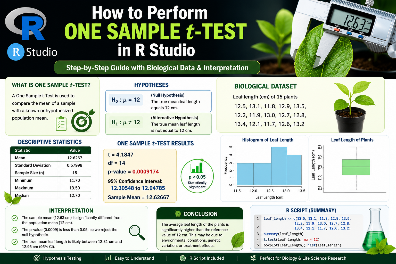
This tutorial demonstrates how to perform a One Sample t-Test in R Studio using a biological dataset containing leaf length measurements from plants. We will cover data preparation, descriptive statistics, hypothesis formulation, execution of the t-test, graphical visualization, and interpretation of the results

Watch Video Tutorial

What is a One Sample t-Test?

A One Sample t-Test is a statistical method used to determine whether the mean of a sample differs significantly from a specified population mean (reference value).

The test compares:

• Sample Mean (observed value)
• Population Mean (expected value)

and determines whether the difference between them is statistically significant.

Formula

$$t=\frac{\bar{x}-\mu}{s/\sqrt{n}}$$

Where:

Symbol	Meaning
$\bar{x}$	Sample Mean
$\mu$	Population Mean
$s$	Sample Standard Deviation
$n$	Sample Size

When Should You Use a One Sample t-Test?

A One Sample t-Test is appropriate when:

• Data are continuous numerical measurements.
• A population or reference mean is known.
• The sample is randomly collected.
• Observations are independent.
• Data are approximately normally distributed.

Biological Examples

• Comparing plant height with a standard variety height.
• Comparing average leaf length with published values.
• Testing whether enzyme activity differs from a reference level.
• Evaluating blood glucose levels against a clinical standard.
• Comparing fish weight against expected population weight.

Biological Dataset Used

The dataset contains leaf length measurements from 15 plants. The values were entered into R Studio using the following vector.

leaf_length <- c(12.5, 13.1, 11.8, 12.9, 13.5,
                 12.2, 11.9, 13.0, 12.7, 12.8,
                 13.4, 12.1, 11.7, 12.6, 13.2)

The objective is to determine whether the average leaf length differs significantly from a reference value of 12 cm.

Step 1: Load the Dataset into R Studio

Create a vector containing the leaf length measurements.

leaf_length <- c(12.5, 13.1, 11.8, 12.9, 13.5,
                 12.2, 11.9, 13.0, 12.7, 12.8,
                 13.4, 12.1, 11.7, 12.6, 13.2)

print(leaf_length)

This command stores the biological measurements and displays them in the console.

Step 2: Generate Descriptive Statistics

Descriptive statistics summarize the central tendency and variability of the data.

summary(leaf_length)

Output obtained from the analysis:

Statistic	Value
Minimum	11.70
1st Quartile	12.15
Median	12.70
Mean	12.63
3rd Quartile	13.05
Maximum	13.50

Interpretation

The average leaf length is approximately 12.63 cm.

The median value is 12.70 cm, which is close to the mean, suggesting that the dataset is relatively symmetrical.

The measurements range from 11.70 cm to 13.50 cm, indicating moderate variability among plants.

Step 3: Calculate Mean, Standard Deviation, and Sample Size

mean_value <- mean(leaf_length)
print(mean_value)

sd_value <- sd(leaf_length)
print(sd_value)

n <- length(leaf_length)
print(n)

Results obtained:

Parameter	Value
Mean	12.62667
Standard Deviation	0.57998
Sample Size	15

Interpretation

The mean leaf length is approximately 12.63 cm.

The standard deviation of 0.58 cm indicates relatively low variation among observations.

The sample contains 15 plants, which is sufficient for demonstrating the One Sample t-Test procedure.

Step 4: Formulate Hypotheses

The reference population mean is set to:$$\mu = 12$$

Null Hypothesis (H₀)

$$H_0 : \mu = 12$$

The true mean leaf length equals 12 cm.

Alternative Hypothesis (H₁)

$$H_1 : \mu \neq 12$$

The true mean leaf length differs from 12 cm.

Step 5: Perform the One Sample t-Test

Execute the following command:

population_mean <- 12

result <- t.test(leaf_length,
                 mu = population_mean)

print(result)

This code compares the observed sample mean against the expected population mean of 12 cm.

One Sample t-Test Output

The output generated from the analysis is shown below.

One Sample t-test

t = 4.1847
df = 14
p-value = 0.0009174

95 percent confidence interval:
12.30548 12.94785

sample estimates:
mean of x = 12.62667

Detailed Interpretation of Results

Sample Mean

The observed sample mean is:$$12.62667$$12.62667

This indicates that the average leaf length of the sampled plants is approximately 12.63 cm.

t Statistic

The calculated t-value is:$$t=4.1847$$

A large t-value indicates that the observed mean differs substantially from the hypothesized population mean relative to the variability present in the dataset.

Degrees of Freedom

$$df=n-1$$$$df=15-1=14$$

The t-distribution used for hypothesis testing is based on 14 degrees of freedom.

p-value

The p-value obtained is:$$0.0009174$$

Since:$$0.0009174 < 0.05$$

the result is statistically significant.

Decision

Reject the null hypothesis.

Confidence Interval

The 95% confidence interval is:$$12.30548\; \text{to}\; 12.94785$$

This interval represents the range within which the true population mean is likely to fall with 95% confidence.

Importantly, the hypothesized mean value of 12 cm does not lie within this interval, further supporting the conclusion that the population mean differs significantly from 12 cm.

Histogram Interpretation

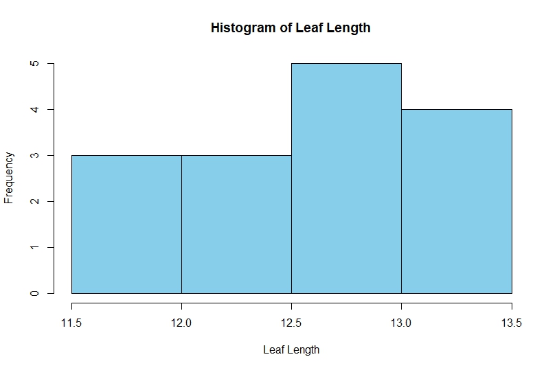
Figure 1. Histogram of Leaf Length Distribution

The histogram shows the frequency distribution of leaf length measurements.

Interpretation

• Values are concentrated between 12 and 13.5 cm.
• No extreme outliers are visible.
• Distribution appears reasonably symmetric.
• Data are approximately normal.

Because the data exhibit an approximately normal distribution, the One Sample t-Test assumptions are reasonably satisfied.

Boxplot Interpretation

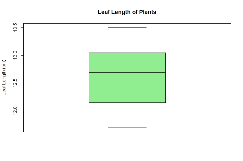
Figure 2. Boxplot of Leaf Length Measurements

The boxplot provides a visual summary of the dataset.

Interpretation

• Median leaf length is approximately 12.7 cm.
• The interquartile range represents the middle 50% of observations.
• No obvious outliers are present.
• Data spread is relatively small.

The absence of extreme observations indicates stable biological measurements.

Complete R Script

The complete R script used for this analysis is provided in the downloadable script file.

Assumptions of One Sample t-Test

Before interpreting results, verify the following assumptions:

1. Continuous Data

Leaf length measurements are continuous numerical variables.

2. Independence

Each plant was measured independently.

3. Normal Distribution

Normality can be assessed using:

shapiro.test(leaf_length)

or by examining:

• Histogram
• Q-Q Plot
• Boxplot

4. Random Sampling

Samples should be collected randomly from the population.

Biological Interpretation

From a biological perspective, the sampled plants exhibit an average leaf length significantly greater than the expected reference value of 12 cm.

Possible biological explanations include:

• Improved nutrient availability.
• Favorable environmental conditions.
• Genetic differences among plants.
• Enhanced irrigation or fertilizer effects.
• Experimental treatment effects.

Further investigation may help identify the factors responsible for the observed increase.

Conclusion

The One Sample t-Test is an essential statistical technique for comparing a sample mean with a known population mean. In this tutorial, we analyzed a biological dataset consisting of plant leaf length measurements and tested whether the average leaf length differed from the reference value of 12 cm. The analysis revealed a statistically significant difference (t = 4.1847, p = 0.0009174), indicating that the true mean leaf length is greater than the expected value. By combining descriptive statistics, hypothesis testing, histograms, boxplots, and confidence intervals, researchers can draw reliable conclusions from biological data using R Studio.