
Introduction
Data visualization is an essential part of data analysis in biology, biostatistics, bioinformatics, agriculture, and medical research. Before performing advanced statistical analyses, researchers often use graphical techniques to understand the distribution and variability of their data.
One of the most effective graphical tools for visualizing data distributions is the box plot, also known as the box-and-whisker plot. A box plot summarizes a dataset using quartiles, median values, spread, and potential outliers, making it easy to compare multiple groups simultaneously.
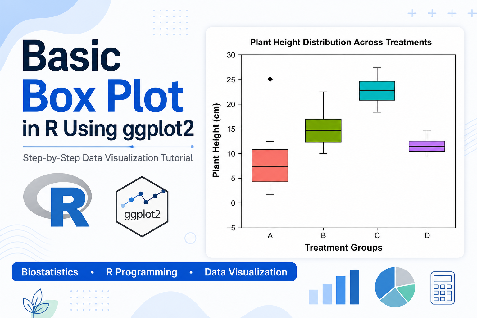
In this tutorial, you will learn how to create a Basic Box Plot in R using the ggplot2 package. We will use a biological dataset representing plant height measurements collected from four treatment groups and explain each step of the R script in detail.
Watch the Video Tutorial
What is a Box Plot?
A box plot is a statistical graph that displays the distribution of numerical data through five important summary statistics:
- Minimum value
- First Quartile (Q1)
- Median (Q2)
- Third Quartile (Q3)
- Maximum value
Additionally, box plots can identify unusual observations known as outliers.
Box plots are widely used because they provide a quick visual summary of data variation and allow easy comparison between groups.
Why Use Box Plots in Biological Research?
Researchers frequently use box plots to:
- Compare treatment effects
- Evaluate experimental results
- Detect outliers
- Assess data variability
- Visualize biological measurements
Common applications include:
- Plant height analysis
- Crop yield comparisons
- Gene expression studies
- Clinical trial data
- Microbiology experiments
- Ecological research
Biological Dataset Used in This Example
The dataset contains plant height measurements collected from four treatment groups:
| Treatment | Description |
|---|---|
| A | Control Group |
| B | Low Fertilizer Dose |
| C | Medium Fertilizer Dose |
| D | High Fertilizer Dose |
The plant height values (cm) are:
| Treatment A | Treatment B | Treatment C | Treatment D |
|---|---|---|---|
| 5 | 10 | 19 | 11 |
| 8 | 12 | 22 | 12 |
| 10 | 15 | 24 | 13 |
| 12 | 18 | 25 | 12 |
| 7 | 16 | 23 | 11 |
| 25 | 14 | 21 | 14 |
| 4 | 22 | 27 | 12 |
Step 1: Load the ggplot2 Package
The first step is to load the ggplot2 package.
library(ggplot2)
The ggplot2 package is one of the most popular visualization libraries in R and is widely used for creating publication-quality graphics.
Step 2: Create the Biological Dataset
Next, create the dataset using the data.frame() function.
bio_data <- data.frame(
  Treatment = c(rep("A",7),
                rep("B",7),
                rep("C",7),
                rep("D",7)),
  Height = c(
    5,8,10,12,7,25,4,
    10,12,15,18,16,14,22,
    19,22,24,25,23,21,27,
    11,12,13,12,11,14,12
  )
)
This code creates two variables:
- Treatment
- Height
Each plant height measurement is assigned to a specific treatment group.
Step 3: Display the Dataset
To verify the data, use:
print(bio_data)
or
View(bio_data)
This helps ensure that the dataset has been entered correctly before creating visualizations.
Step 4: Create the Basic Box Plot
The following code creates the box plot:
ggplot(bio_data,
       aes(x = Treatment,
           y = Height,
           fill = Treatment)) +
  geom_boxplot()
This produces a basic box plot with separate colored boxes for each treatment group.
Step 5: Add Titles and Axis Labels
To improve readability:
labs(
  title = "Plant Height Distribution Across Treatments",
  x = "Treatment Groups",
  y = "Plant Height (cm)"
)
These labels help readers understand the variables displayed in the graph.
Step 6: Customize the Appearance
The script uses:
theme_bw()
This provides:
- White background
- Clean appearance
- Professional formatting
The script also removes:
legend.position = "none"
because treatment groups are already labeled on the x-axis.
Understanding the Components of a Box Plot
A box plot contains several important elements.
Median
The horizontal line inside the box represents the median.
The median indicates the center of the dataset.
First Quartile (Q1)
The bottom edge of the box represents Q1.
25% of observations lie below this value.
Third Quartile (Q3)
The upper edge of the box represents Q3.
75% of observations lie below this value.
Interquartile Range (IQR)
The box itself represents:
IQR = Q3 − Q1
The IQR contains the middle 50% of observations.
Whiskers
The whiskers extend from the box and show the range of most observations.
Outliers
Points outside the whiskers are considered outliers.
In Treatment A, the value 25 cm appears as an outlier.
Outliers may indicate:
- Biological variation
- Measurement errors
- Experimental anomalies
Interpretation of the Box Plot
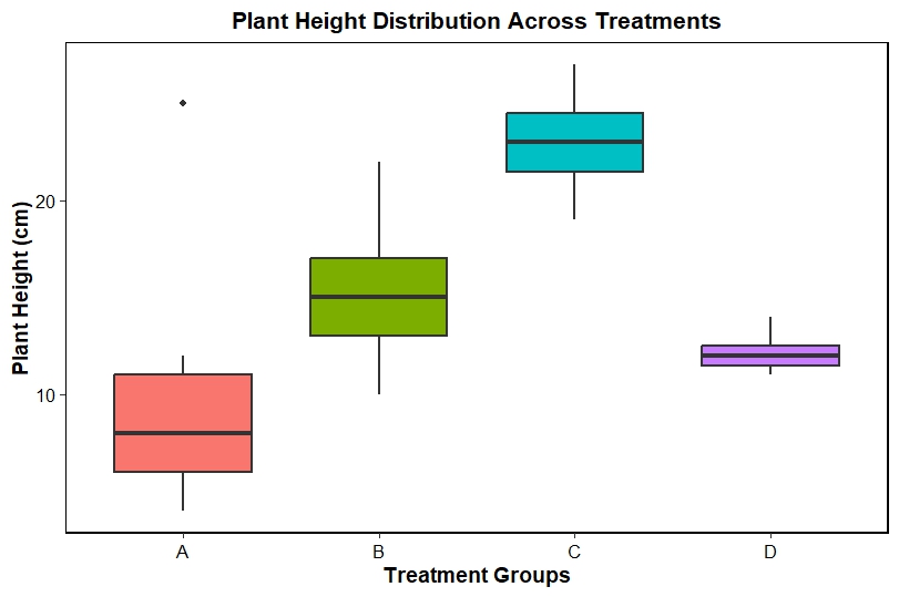
Treatment A
- Median height around 8 cm
- Largest variability
- Contains a high outlier
- Indicates inconsistent plant growth
Treatment B
- Median height around 15 cm
- Moderate variability
- Better growth than Treatment A
Treatment C
- Highest median height
- Best plant growth performance
- Moderate variation
Treatment D
- Median around 12 cm
- Lowest variability
- Most consistent plant growth
What Does This Result Mean?
The box plot suggests that Treatment C produced the tallest plants overall.
Treatment D generated more consistent results, while Treatment A exhibited substantial variation and contained an outlier.
If these treatments represented fertilizer concentrations, the results would suggest that the medium fertilizer dose (Treatment C) provided the most effective growth response.
Advantages of Box Plots
Box plots offer several benefits:
- Easy to create
- Summarize large datasets
- Detect outliers quickly
- Compare multiple groups simultaneously
- Require minimal space
- Useful for publication-quality figures
Common Applications of Box Plots
Researchers use box plots in:
Biology
Comparing plant growth under different treatments.
Agriculture
Evaluating fertilizer effects on crop yield.
Medicine
Comparing patient responses to treatments.
Bioinformatics
Analyzing gene expression levels.
Ecology
Comparing species abundance across habitats.
Conclusion
A box plot is one of the most powerful and widely used statistical visualization tools for exploratory data analysis. Using the ggplot2 package in R, researchers can quickly create professional-quality box plots to compare groups, identify outliers, and understand data distributions. In this example, plant height measurements from four treatment groups were visualized and interpreted effectively. Treatment C demonstrated the highest growth performance, while Treatment D showed the most consistent results. Whether you work in biology, agriculture, medicine, bioinformatics, or biostatistics, mastering box plots in R is an essential skill for analyzing and communicating scientific data.